Gaussian Laser Profile#

class lasy.profiles.GaussianProfile(wavelength, pol, laser_energy, w0, tau, t_peak, x0=0, y0=0, cep_phase=0, z_foc=0, phi2=0, beta=0, zeta=0, stc_theta=0)[source]#

Class for the analytic profile of a Gaussian laser pulse.

More precisely, the electric field corresponds to:

\[E_u(\boldsymbol{x}_\perp,t) = Re\left[ E_0\, \exp\left( -\frac{\boldsymbol{x}_\perp^2}{w_0^2} - \frac{(t-t_{peak})^2}{\tau^2} -i\omega_0(t-t_{peak}) + i\phi_{cep}\right) \times p_u \right]\]

where \(u\) is either \(x\) or \(y\), \(p_u\) is the polarization vector, \(Re\) represent the real part, and \(\boldsymbol{x}_\perp\) is the transverse coordinate (orthogonal to the propagation direction). The other parameters in this formula are defined below. This profile also supports some chirp parameters that are omitted in the expression above for clarity.

Parameters:

wavelengthfloat (in meter): The main laser wavelength \(\lambda_0\) of the laser, which defines \(\omega_0\) in the above formula, according to \(\omega_0 = 2\pi c/\lambda_0\).
pollist of 2 complex numbers (dimensionless): Polarization vector. It corresponds to \(p_u\) in the above formula ; \(p_x\) is the first element of the list and \(p_y\) is the second element of the list. Using complex numbers enables elliptical polarizations.
laser_energyfloat (in Joule): The total energy of the laser pulse. The amplitude of the laser field (\(E_0\) in the above formula) is automatically calculated so that the pulse has the prescribed energy.
w0float (in meter): The waist of the laser pulse, i.e. \(w_0\) in the above formula.
taufloat (in second): The duration of the laser pulse, i.e. \(\tau\) in the above formula. Note that \(\tau = \tau_{FWHM}/\sqrt{2\log(2)}\), where \(\tau_{FWHM}\) is the Full-Width-Half-Maximum duration of the intensity distribution of the pulse.
t_peakfloat (in second): The time at which the laser envelope reaches its maximum amplitude, i.e. \(t_{peak}\) in the above formula.
x0 , y0float (in meter) optional (default: ‘0’): Transverse centroid for the laser pulse
cep_phasefloat (in radian), optional: The Carrier Envelope Phase (CEP), i.e. \(\phi_{cep}\) in the above formula (i.e. the phase of the laser oscillation, at the time where the laser envelope is maximum)
z_focfloat (in meter), optional: Position of the focal plane. (The laser pulse is initialized at z=0.)
phi2float (in second^2), optional (default: ‘0’): The group-delay dispersion defined as \(\phi^{(2)} = \frac{dt_0}{d\omega}\). Here \(t_0\) is the temporal position of this frequency component.
betafloat (in second), optional (default: ‘0’): The angular dispersion defined as \(\beta = \frac{d\theta_0}{d\omega}\). Here \(\theta_0\) is the propagation angle of this frequency component.
zetafloat (in meter * second), optional (default: ‘0’): A spatial chirp defined as \(\zeta = \frac{dx_0}{d\omega}\). Here \(x_0\) is the transverse beam center position of this frequency component. The definitions of beta, phi2, and zeta are taken from [S. Akturk et al., Optics Express 12, 4399 (2004)].
stc_thetafloat (in radian), optional (default: ‘0’): Transverse direction along which there are chirps and spatio-temporal couplings. A value of 0 corresponds to the x-axis.

Examples

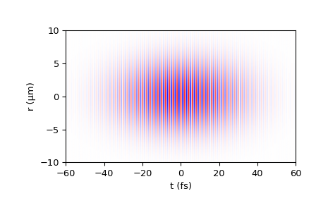
>>> import matplotlib.pyplot as plt
>>> from lasy.backend import xp, to_cpu
>>> from lasy.laser import Laser
>>> from lasy.profiles.gaussian_profile import GaussianProfile
>>> from lasy.utils.laser_utils import get_full_field
>>> # Create profile.
>>> profile = GaussianProfile(
...     wavelength=0.6e-6,  # m
...     pol=(1, 0),
...     laser_energy=1.0,  # J
...     w0=5e-6,  # m
...     tau=30e-15,  # s
...     t_peak=0.0,  # s
... )
>>> # Create laser with given profile in `rt` geometry.
>>> laser = Laser(
...     dim="rt",
...     lo=(0e-6, -60e-15),
...     hi=(10e-6, +60e-15),
...     npoints=(50, 400),
...     profile=profile,
... )
>>> # Visualize field.
>>> E_rt, extent = get_full_field(laser)
>>> extent[2:] *= 1e6
>>> extent[:2] *= 1e15
>>> tmin, tmax, rmin, rmax = extent
>>> vmax = xp.abs(E_rt).max()
>>> plt.imshow(
...     to_cpu(E_rt),
...     origin="lower",
...     aspect="auto",
...     vmax=vmax,
...     vmin=-vmax,
...     extent=[tmin, tmax, rmin, rmax],
...     cmap="bwr",
... )
>>> plt.xlabel("t (fs)")
>>> plt.ylabel("r (µm)")

evaluate(x, y, t)[source]#

Return the longitudinal envelope.

Parameters:

tndarrays of floats: Define longitudinal points on which to evaluate the envelope
x,yndarrays of floats: Define transverse points on which to evaluate the envelope

Returns:

envelopendarray of complex numbers: Contains the value of the longitudinal envelope at the specified points. This array has the same shape as the array t.