Laser Pulse in Space Only

In this example we look at the special case where one is only interested in defining and manipulating the spatial profile of the laser pulse. In this case, having a full 3D or quasi-3D profile is an inefficient use of resources. For this purpose, we have defined the longitudinal laser profile ContinuousWaveProfile which allows one to treat the longitudinal profile as a 1 pixel continuous wave laser in time.

Generate a Gaussian Profile in Space with a Continuous Wave Longitudinal Profile

One key difference you might notice to the traditional definition of the laser pulse is that we do not use the laser energy to scale the amplitude of the electric field, but in this case we use the peak intensity of the laser pulse

import matplotlib.pyplot as plt
from scipy.constants import c, epsilon_0

from lasy.backend import to_cpu, xp
from lasy.laser import Laser
from lasy.profiles import CombinedLongitudinalTransverseProfile
from lasy.profiles.longitudinal import ContinuousWaveProfile
from lasy.profiles.transverse import GaussianTransverseProfile
from lasy.utils.laser_utils import compute_laser_energy, get_w0

# Physical Parameters
peak_fluence = 1.0e4  # J/m^2
spot_size = 10e-3
wavelength = 800e-9
pol = (1, 0)

long_prof = ContinuousWaveProfile(wavelength)
tran_prof = GaussianTransverseProfile(spot_size)
profile = CombinedLongitudinalTransverseProfile(
    wavelength, pol, long_prof, tran_prof, peak_fluence=peak_fluence
)

LASY: using backend NP

Define the Computational Grid

Here we should note the the lo and hi variables have been passed as None for the longitudinal axis as it is a continuous wave laser. Additionally, the number of points along the longitudinal dimension is 1.

# Computational Grid
dim = "xyt"
lo = (-5 * spot_size, -5 * spot_size, None)
hi = (5 * spot_size, 5 * spot_size, None)
npoints = (1000, 1000, 1)

laser = Laser(dim, lo, hi, npoints, profile)

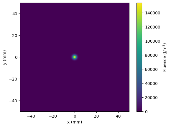
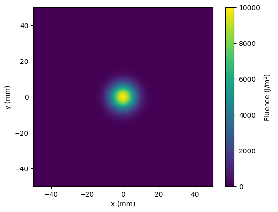
laser.show()

Visualizing and Analyzing the Pulse

We see that the standard laser.show() command works here and we indeed get a laser which is invariant in time.

One can also extract the laser intensity and use this to visualize the pule.

intensity = epsilon_0 * c / 2 * xp.abs(laser.grid.get_temporal_field()) ** 2
fluence = xp.sum(intensity, axis=-1) * laser.grid.dx[-1]
extent = (
    laser.grid.axes[0].min() * 1e3,
    laser.grid.axes[0].max() * 1e3,
    laser.grid.axes[1].min() * 1e3,
    laser.grid.axes[1].max() * 1e3,
)
plt.figure()
plt.imshow(to_cpu(fluence), extent=extent)
plt.xlabel("x (mm)")
plt.ylabel("y (mm)")
plt.colorbar(label=r"Fluence (J/m$^2$)")

<matplotlib.colorbar.Colorbar at 0x754e9461f0d0>

Adding Optics

Optics can be added in the usual way to manipulate the laser pulse. Additionally, standard laser_utils functions work out of the box.

Also for this kind of beam, the propagators may be used.

w0_meas = get_w0(laser.grid, laser.dim)
energy0_meas = compute_laser_energy(laser.dim, laser.grid)

from lasy.optical_elements import ParabolicMirror

focal_length = 100
oap = ParabolicMirror(focal_length)

laser.apply_optics(oap)
laser.propagate(focal_length)

w1_meas = get_w0(laser.grid, laser.dim)
w1_expt = 2 * xp.sqrt(2) / xp.pi * wavelength * focal_length / (2 * spot_size)
energy1_meas = compute_laser_energy(laser.dim, laser.grid)


print("Initial Spot Size = %.2f mm" % (w0_meas * 1e3))
print("Final Spot Size    = %.2f mm" % (w1_meas * 1e3))
print("Expected Final Spot Size = %.2f mm" % (w1_meas * 1e3))
print("Initial Pulse Energy = %.2f J" % (energy0_meas))
print("Final Pulse Energy   = %.2f J" % (energy1_meas))

Available backends are: NP
NP is chosen
Initial Spot Size = 10.00 mm
Final Spot Size    = 2.55 mm
Expected Final Spot Size = 2.55 mm
Initial Pulse Energy = 1.57 J
Final Pulse Energy   = 1.57 J

intensity = epsilon_0 * c / 2 * xp.abs(laser.grid.get_temporal_field()) ** 2
fluence = xp.sum(intensity, axis=-1) * laser.grid.dx[-1]
extent = (
    laser.grid.axes[0].min() * 1e3,
    laser.grid.axes[0].max() * 1e3,
    laser.grid.axes[1].min() * 1e3,
    laser.grid.axes[1].max() * 1e3,
)
plt.figure()
plt.imshow(to_cpu(fluence), extent=extent)
plt.xlabel("x (mm)")
plt.ylabel("y (mm)")
plt.colorbar(label=r"Fluence (J/m$^2$)")

<matplotlib.colorbar.Colorbar at 0x754e946717d0>