Collins propagator and focal scan

In this tutorial, we simulate the propagation of a focusing continuous-wave (CW) beam in free-space. This gives an overview of the functionality of the CollinsSFFTPropagator class which defines a diffraction integral expressed in terms of an optical ray matrix. The optical ray matrix is defined in the ABCD class.

The CollinsSFFTPropagator is based on a single fast-Fourier transform (SFFT) and is used to go between the near-field (NF) and the far-field (FF) in imaging systems.

This tutorial gives an overview of how to use ABCD to define the optical ray matrices for basic components such as thin-lenses and drift sections in vacuum. A Gaussian continous wave (CW) beam is propagated to the first plane of the focal scan using the CollinsSFFTPropagator, using a lens and free-space drift defined with ABCD matrices. This is repeated for subsequent planes in the focal scan.

First we import a few relevant modules:

import copy

import matplotlib.pyplot as plt
from mpl_toolkits.axes_grid1 import make_axes_locatable
from scipy.constants import c, epsilon_0

from lasy.backend import to_cpu, xp
from lasy.laser import Laser
from lasy.profiles import CombinedLongitudinalTransverseProfile
from lasy.profiles.longitudinal import ContinuousWaveProfile
from lasy.profiles.transverse import GaussianTransverseProfile
from lasy.propagators import ABCD, CollinsSFFTPropagator

LASY: using backend NP

Next, we define the beam to be CW with a tophat profile in the transverse plane:

peak_fluence = 1.0e4  # J/m^2
spot_size = 10e-3
wavelength = 800e-9
omega0 = 2 * xp.pi * c / wavelength
pol = (1, 0)

long_prof = ContinuousWaveProfile(wavelength)
tran_prof = GaussianTransverseProfile(spot_size)
laser_profile = CombinedLongitudinalTransverseProfile(
    wavelength, pol, long_prof, tran_prof, peak_fluence=peak_fluence
)

We now define the grids at the input plane and the full laser object in terms of the grid and the laser:

dimensions = "xyt"  # Use cylindrical geometry
lo = (-15.0 * spot_size, -15.0 * spot_size, None)  # Lower bounds of the simulation box
hi = (15.0 * spot_size, 15.0 * spot_size, None)  # Upper bounds of the simulation box
num_points = (256, 256, 1)  # Number of points in each dimension

laser = Laser(dimensions, lo, hi, num_points, laser_profile)
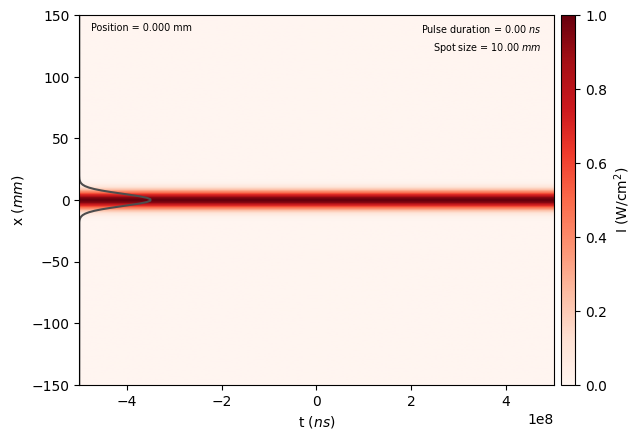
laser.show(envelope_type="intensity")  # In this case this is the fluence (CW beam)

We will now set up the focal scan by estimating the Rayleigh length and using this to define the axial grid:

focal_length = 300e-3
z_R = focal_length**2 / (
    xp.pi * spot_size**2 / wavelength
)  # The estimated Rayleigh length after the lens
spot_size_focus = (
    laser.profile.lambda0 * focal_length / (xp.pi * spot_size)
)  # Estimated focal spot-size after the lens
limits = [-10.0 * z_R, 10.0 * z_R]  # Set the depth limits for the focal scan
N_points = 200

# Estimate of fluence at input plane and focus (assuming a Gaussian pulse)
E_0 = peak_fluence * xp.pi * spot_size**2 / 2
print(E_0)
F_in = 2.0 * E_0 / (xp.pi * (spot_size) ** 2) / 1e4
F_out = 2.0 * E_0 / (xp.pi * (spot_size_focus) ** 2) / 1e4
print(
    "Fluence at input plane [J cm-2]: %0.1e" % (F_in),
    "\nFluence at focus [J cm-2]: %0.1e" % (F_out),
)

z_grid = (
    xp.linspace(limits[0], limits[1], N_points) + focal_length
)  # Absolute axial distances from the input plane of the lens

1.5707963267948968
Fluence at input plane [J cm-2]: 1.0e+00
Fluence at focus [J cm-2]: 1.7e+06

We will now make a copy of the laser and define both the SFFT propagator that we will use in our focal scan. We then initialise the ABCD matrix and add a thin-lens of the correct focal length:

prop = CollinsSFFTPropagator(dimensions, omega0)
abcd = ABCD()
abcd.add_lens(focal_length)

Now we will perform the focal scan (see comments within the loop for an explanation of intermediate steps):

focal_scan = []  # Create empty list to store the focal scan data

for i, z in enumerate(z_grid):
    laser_input = copy.deepcopy(laser)
    if i == 0:
        abcd.add_vacuum(z)
        prop.propagate(laser_input.grid, abcd)
        grid_out = laser_input.grid
    else:
        abcd.add_vacuum(z - z_grid[i - 1])
        prop.propagate(laser_input.grid, abcd, grid_out=grid_out)

    focal_scan.append(laser_input)  # Storing the full focal scan data

    field = laser_input.grid.get_temporal_field()[
        num_points[0] // 2, :, num_points[2] // 2
    ]
    lineout = epsilon_0 * c / 2 * xp.abs(field) ** 2 / 1e4

    # Stack these lineouts to plot a cross-section of the focal scan
    if i == 0:
        scanImg = lineout
    else:
        scanImg = xp.vstack((scanImg, lineout))

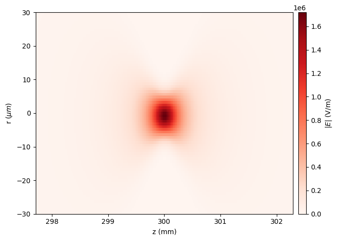
We will now get the output grids from the simulation and plot a cross-section of the focal scan

# Get the grids from the simulation
x_grid = focal_scan[0].grid.axes[
    0
]  # Output axes as automatically calculated by the CollinsSFFTPropagator
y_grid = focal_scan[0].grid.axes[1]
extent = [z_grid[0] * 1e3, z_grid[-1] * 1e3, y_grid[0] * 1e6, y_grid[-1] * 1e6]

# Make plot of focal scan cross-section
fig, ax = plt.subplots(1, 1, figsize=(7, 5), tight_layout=True)
ax_divider = make_axes_locatable(ax)
im = ax.imshow(
    to_cpu(scanImg.T), aspect="auto", interpolation="none", cmap="Reds", extent=extent
)
cax = ax_divider.append_axes("right", size="3%", pad="2%")
cb = fig.colorbar(im, cax=cax)
cb.set_label(r"$|E|$ (V/m)")
ax.set_xlabel("z (mm)")
ax.set_ylabel(r"r ($\mu m$)")
ax.set_ylim(-30, 30)
plt.show()