Initializing a flying-focus laser from an axiparabola#
In this example, we generate a “flying-focus” laser from an axiparabola. This is done by sending a super-Gaussian laser (in the near-field) onto an axiparabola and propagating it to the far field.
Generate a super-Gaussian laser#
Define the physical profile, as combination of a longitudinal and transverse profile.
[1]:
from lasy.laser import Laser
from lasy.profiles.combined_profile import CombinedLongitudinalTransverseProfile
from lasy.profiles.longitudinal import GaussianLongitudinalProfile
from lasy.profiles.transverse import SuperGaussianTransverseProfile

wavelength = 800e-9  # Laser wavelength in meters
polarization = (1, 0)  # Linearly polarized in the x direction
energy = 1.5  # Energy of the laser pulse in joules
spot_size = 1e-3  # Spot size in the near-field: millimeter-scale
pulse_duration = 30e-15  # Pulse duration of the laser in seconds
t_peak = 0.0  # Location of the peak of the laser pulse in time

laser_profile = CombinedLongitudinalTransverseProfile(
    wavelength,
    polarization,
    GaussianLongitudinalProfile(wavelength, pulse_duration, t_peak),
    SuperGaussianTransverseProfile(spot_size, n_order=16),
    laser_energy=energy,
)
LASY: using backend NP
Define the grid on which this profile is evaluated.
The grid needs to be wide enough to contain the millimeter-scale spot size, but also fine enough to resolve the micron-scale laser wavelength.
[2]:
dimensions = "rt" # Use cylindrical geometry
lo = (0, -2.5 * pulse_duration) # Lower bounds of the simulation box
hi = (1.1 * spot_size, 2.5 * pulse_duration) # Upper bounds of the simulation box
num_points = (3000, 30) # Number of points in each dimension
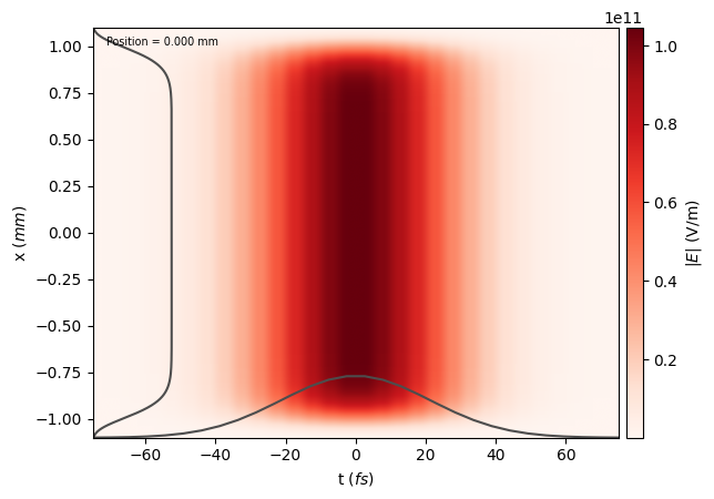
laser = Laser(dimensions, lo, hi, num_points, laser_profile)
[3]:
laser.show()
Propagate the laser through the axiparabola, and to the far field.#
First, define the parameters of the axiparabola.
[4]:
from lasy.optical_elements import Axiparabola

f0 = 3e-2  # Focal distance
delta = 1.5e-2  # Focal range
R = spot_size  # Radius
axiparabola = Axiparabola(f0, delta, R)
Apply the effect of the axiparabola, and then propagate the laser for a distance z=f0 (beginning of the focal range).
[5]:
laser.apply_optics(axiparabola)
laser.propagate(f0)
Available backends are: NP
NP is chosen
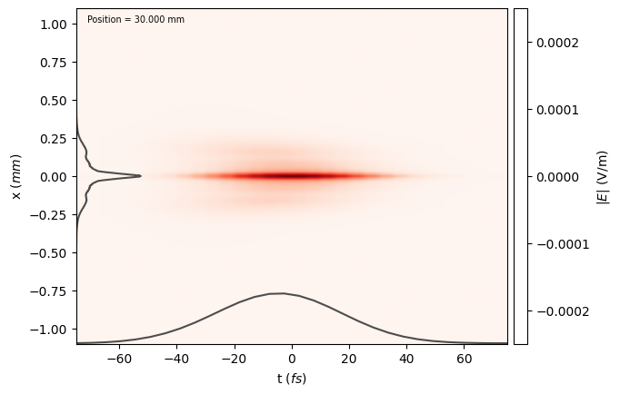
[6]:
import matplotlib.pyplot as plt

laser.show()
plt.ylim(-0.25e-3, 0.25e-3)
[6]:
(-0.00025, 0.00025)
At this point, the laser can be saved to file, and used e.g. as input to a PIC simulation.
[7]:
laser.write_to_file("flying_focus", "h5")
Check that the electric field on axis remains high over many Rayleigh ranges#
An axiparabola can maintain a high laser field over a long distance (larger than the Rayleigh length). Here, we can check that the laser field remains high over several Rayleigh length.
[8]:
import math

ZR = math.pi * wavelength * f0**2 / spot_size**2
print("Rayleigh length: %.f mm" % (1.0e3 * ZR))
print("Focal range: %.f mm" % (1.0e3 * delta))
Rayleigh length: 2 mm
Focal range: 15 mm
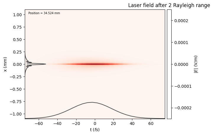
[9]:
laser.propagate(2 * ZR)
laser.show()
plt.ylim(-0.25e-3, 0.25e-3)
plt.title("Laser field after 2 Rayleigh range")
[9]:
Text(0.5, 1.0, 'Laser field after 2 Rayleigh range')
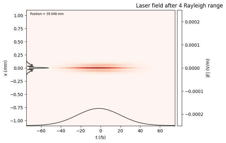
[10]:
laser.propagate(2 * ZR)
laser.show()
plt.ylim(-0.25e-3, 0.25e-3)
plt.title("Laser field after 4 Rayleigh range")
[10]:
Text(0.5, 1.0, 'Laser field after 4 Rayleigh range')