Laser Pulse in Time Only

In this example we look at the special case where one is only interested in defining and manipulating the temporal profile of the laser pulse. In this case, having a full 3D or quasi-3D profile is an inefficient use of resources. For this purpose, we have defined the transverse laser profile PlaneWaveProfile which allows one to treat the transverse profile as a 1 pixel plane wave.

Generate a Gaussian Profile in Time with a Plane Wave Transverse Profile

One key difference you might notice to the traditional definition of the laser pulse is that we do not use the laser energy to scale the amplitude of the electric field, but in this case we use the peak power of the laser pulse

import matplotlib.pyplot as plt
import numpy as np
from scipy.constants import c

from lasy.laser import Laser
from lasy.profiles import CombinedLongitudinalTransverseProfile
from lasy.profiles.longitudinal import GaussianLongitudinalProfile
from lasy.profiles.transverse import PlaneWaveProfile
from lasy.utils.laser_utils import get_duration, get_laser_fluence, get_laser_power

# Physical Parameters
tau = 30e-15
wavelength = 800e-9
t_peak = 0.0
pol = (1, 0)
peak_power = 1e12  # W

long_prof = GaussianLongitudinalProfile(wavelength, tau, t_peak)
tran_prof = PlaneWaveProfile()
profile = CombinedLongitudinalTransverseProfile(
    wavelength, pol, long_prof, tran_prof, peak_power=peak_power
)

Define the Computational Grid

Here we should note the the lo and hi variables have been passed as None for the transverse axes as it is a plane wave. Additionally, the number of points along the transverse dimensions is 1 in each direction.

# Computational Grid
dim = "xyt"
lo = (None, None, -5 * tau)
hi = (None, None, 5 * tau)
npoints = (1, 1, 1000)

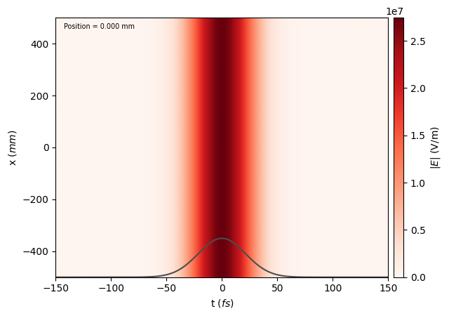
laser = Laser(dim, lo, hi, npoints, profile)

laser.show()

Visualizing and Analyzing the Pulse

We see that the standard laser.show() command works here and we indeed get a plane wave.

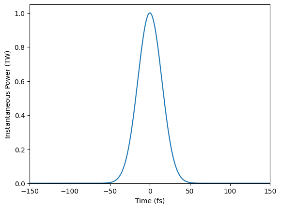
One can also extract the laser power and use this to visualize the pule.

power = get_laser_power(laser.dim, laser.grid)

plt.figure()
plt.plot(laser.grid.axes[-1] * 1e15, power / 1e12)
plt.xlim(laser.grid.axes[-1][0] * 1e15, laser.grid.axes[-1][-1] * 1e15)
plt.ylim(0, None)
plt.xlabel("Time (fs)")
plt.ylabel("Instantaneous Power (TW)")

Text(0, 0.5, 'Instantaneous Power (TW)')

Adding Optics

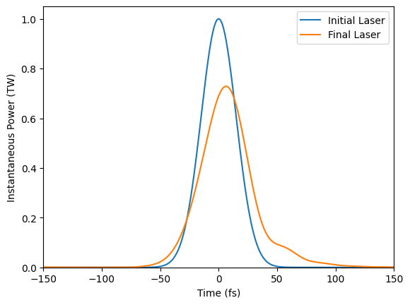
Optics can be added in the usual way to manipulate the laser pulse. Additionally, standard laser_utils functions work out of the box

tau0_meas = get_duration(laser.grid, laser.dim)
fluence0_meas = get_laser_fluence(laser.grid)

from lasy.optical_elements import PolynomialSpectralPhase

omega0 = 2 * np.pi * c / wavelength
gdd = 500e-30
tod = 15000e-45
dazzler = PolynomialSpectralPhase(omega0, gdd=gdd, tod=tod)

laser.apply_optics(dazzler)

tau1_meas = get_duration(laser.grid, laser.dim)
fluence1_meas = get_laser_fluence(laser.grid)


print("Initial Pulse Duration = %.2f fs" % (tau0_meas * 1e15))
print("Final Pulse Duration   = %.2f fs" % (tau1_meas * 1e15))
print("Initial Pulse Fluence = %.2e mJ/cm2" % (fluence0_meas / 10))
print("Final Pulse Fluence  = %.2e mJ/cm2" % (fluence1_meas / 10))

Initial Pulse Duration = 15.00 fs
Final Pulse Duration   = 25.26 fs
Initial Pulse Fluence = 3.76e-03 mJ/cm2
Final Pulse Fluence  = 3.76e-03 mJ/cm2

power1 = get_laser_power(laser.dim, laser.grid)

plt.figure()
plt.plot(laser.grid.axes[-1] * 1e15, power / 1e12, label="Initial Laser")
plt.plot(laser.grid.axes[-1] * 1e15, power1 / 1e12, label="Final Laser")
plt.xlim(laser.grid.axes[-1][0] * 1e15, laser.grid.axes[-1][-1] * 1e15)
plt.ylim(
    0,
)
plt.xlabel("Time (fs)")
plt.ylabel("Instantaneous Power (TW)")
plt.legend()

<matplotlib.legend.Legend at 0x7d12fb25e610>