Collins propagator and focal scan

In this tutorial, we simulate the propagation of a focusing continuous-wave (CW) beam in free-space. This gives an overview of the functionality of the CollinsSFFTPropagator class which defines a diffraction integral expressed in terms of an optical ray matrix. The optical ray matrix is defined in the ABCD class.

The CollinsSFFTPropagator is based on a single fast-Fourier transform (SFFT) and is used to go between the near-field (NF) and the far-field (FF) in imaging systems.

This tutorial gives an overview of how to use ABCD to define the optical ray matrices for basic components such as thin-lenses and drift sections in vacuum. A Gaussian continous wave (CW) beam is propagated to the first plane of the focal scan using the CollinsSFFTPropagator, using a lens and free-space drift defined with ABCD matrices. This is repeated for subsequent planes in the focal scan.

First we import a few relevant modules:

import copy

import matplotlib.pyplot as plt
import numpy as np
from mpl_toolkits.axes_grid1 import make_axes_locatable
from scipy.constants import c, epsilon_0

from lasy.laser import Laser
from lasy.profiles import CombinedLongitudinalTransverseProfile
from lasy.profiles.longitudinal import ContinuousWaveProfile
from lasy.profiles.transverse import GaussianTransverseProfile
from lasy.propagators import ABCD, CollinsSFFTPropagator

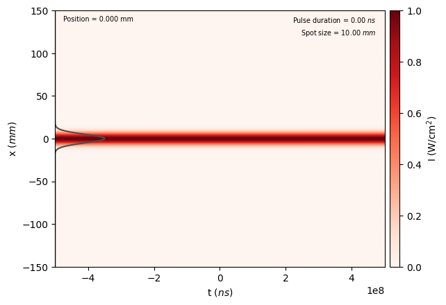
Next, we define the beam to be CW with a tophat profile in the transverse plane:

peak_fluence = 1.0e4  # J/m^2
spot_size = 10e-3
wavelength = 800e-9
omega0 = 2 * np.pi * c / wavelength
pol = (1, 0)

long_prof = ContinuousWaveProfile(wavelength)
tran_prof = GaussianTransverseProfile(spot_size)
laser_profile = CombinedLongitudinalTransverseProfile(
    wavelength, pol, long_prof, tran_prof, peak_fluence=peak_fluence
)

We now define the grids at the input plane and the full laser object in terms of the grid and the laser:

dimensions = "xyt"  # Use cylindrical geometry
lo = (-15.0 * spot_size, -15.0 * spot_size, None)  # Lower bounds of the simulation box
hi = (15.0 * spot_size, 15.0 * spot_size, None)  # Upper bounds of the simulation box
num_points = (256, 256, 1)  # Number of points in each dimension

laser = Laser(dimensions, lo, hi, num_points, laser_profile)
laser.show(envelope_type="intensity")  # In this case this is the fluence (CW beam)

We will now set up the focal scan by estimating the Rayleigh length and using this to define the axial grid:

focal_length = 300e-3
z_R = focal_length**2 / (
    np.pi * spot_size**2 / wavelength
)  # The estimated Rayleigh length after the lens
spot_size_focus = (
    laser.profile.lambda0 * focal_length / (np.pi * spot_size)
)  # Estimated focal spot-size after the lens
limits = [-10.0 * z_R, 10.0 * z_R]  # Set the depth limits for the focal scan
N_points = 200

# Estimate of fluence at input plane and focus (assuming a Gaussian pulse)
E_0 = peak_fluence * np.pi * spot_size**2 / 2
print(E_0)
F_in = 2.0 * E_0 / (np.pi * (spot_size) ** 2) / 1e4
F_out = 2.0 * E_0 / (np.pi * (spot_size_focus) ** 2) / 1e4
print(
    "Fluence at input plane [J cm-2]: %0.1e" % (F_in),
    "\nFluence at focus [J cm-2]: %0.1e" % (F_out),
)

z_grid = (
    np.linspace(limits[0], limits[1], N_points) + focal_length
)  # Absolute axial distances from the input plane of the lens

1.5707963267948968
Fluence at input plane [J cm-2]: 1.0e+00
Fluence at focus [J cm-2]: 1.7e+06

We will now make a copy of the laser and define both the SFFT propagator that we will use in our focal scan. We then initialise the ABCD matrix and add a thin-lens of the correct focal length:

prop = CollinsSFFTPropagator(dimensions, omega0)
abcd = ABCD()
abcd.add_lens(focal_length)

Now we will perform the focal scan (see comments within the loop for an explanation of intermediate steps):

focal_scan = []  # Create empty list to store the focal scan data

for i, z in enumerate(z_grid):
    laser_input = copy.deepcopy(laser)
    if i == 0:
        abcd.add_vacuum(z)
        prop.propagate(laser_input.grid, abcd)
        grid_out = laser_input.grid
    else:
        abcd.add_vacuum(z - z_grid[i - 1])
        prop.propagate(laser_input.grid, abcd, grid_out=grid_out)

    focal_scan.append(laser_input)  # Storing the full focal scan data

    field = laser_input.grid.get_temporal_field()[
        num_points[0] // 2, :, num_points[2] // 2
    ]
    lineout = epsilon_0 * c / 2 * np.abs(field) ** 2 / 1e4

    # Stack these lineouts to plot a cross-section of the focal scan
    if i == 0:
        scanImg = lineout
    else:
        scanImg = np.vstack((scanImg, lineout))

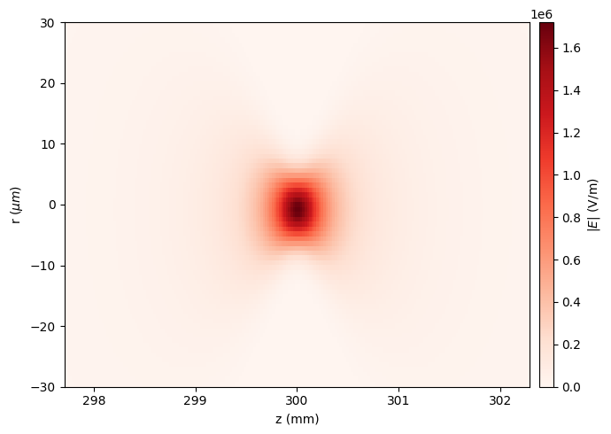
We will now get the output grids from the simulation and plot a cross-section of the focal scan

# Get the grids from the simulation
x_grid = focal_scan[0].grid.axes[
    0
]  # Output axes as automatically calculated by the CollinsSFFTPropagator
y_grid = focal_scan[0].grid.axes[1]
extent = [z_grid[0] * 1e3, z_grid[-1] * 1e3, y_grid[0] * 1e6, y_grid[-1] * 1e6]

# Make plot of focal scan cross-section
fig, ax = plt.subplots(1, 1, figsize=(7, 5), tight_layout=True)
ax_divider = make_axes_locatable(ax)
im = ax.imshow(
    scanImg.T, aspect="auto", interpolation="none", cmap="Reds", extent=extent
)
cax = ax_divider.append_axes("right", size="3%", pad="2%")
cb = fig.colorbar(im, cax=cax)
cb.set_label(r"$|E|$ (V/m)")
ax.set_xlabel("z (mm)")
ax.set_ylabel(r"r ($\mu m$)")
ax.set_ylim(-30, 30)
plt.show()