Laser from longitudinal and transverse profiles#
In this tutorial, you will learn to create a Laser from an experimental measurement of the laser spectrum and a 2D image of the transverse intensity profile. We’ll start by loading all packages required.
[1]:
import matplotlib.pyplot as plt
import numpy as np
from mpl_toolkits.axes_grid1 import make_axes_locatable
from PIL import Image

from lasy.laser import Laser
from lasy.profiles.combined_profile import CombinedLongitudinalTransverseProfile
from lasy.profiles.longitudinal import LongitudinalProfileFromData
from lasy.profiles.transverse import TransverseProfileFromData
from lasy.profiles.transverse.hermite_gaussian_profile import (
    HermiteGaussianTransverseProfile,
)
from lasy.utils.mode_decomposition import hermite_gauss_decomposition
Next, let’s define the physical parameters defining our laser pulse.
[2]:
polarization = (1, 0)  # Linearly polarized in the x direction
energy_J = 1  # Pulse energy in Joules
cal = 0.2e-6  # Camera pixel size in meters. Used for calibration
In what follows, we do a few steps to create a LASY profile. Profile is the object used in LASY to describe the properties of the pulse. This profile is then used to create a Laser object, i.e., a regular mesh with the values of the vector potential of the pulse. This mesh can be 3D for a 3D (xyt) geometry, or can consist of a few 2D grids for cylindrical geometry with mode decomposition.
Reconstruct longitudinal profile#
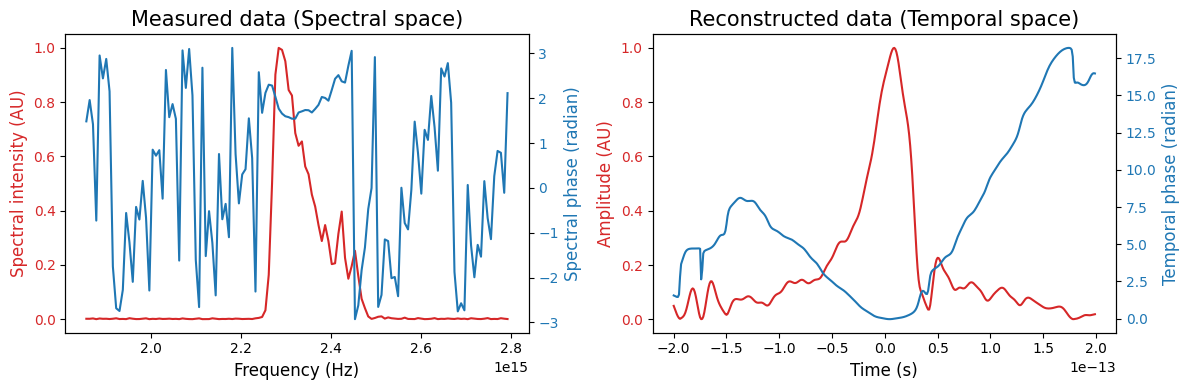
We start from an example dataset obtained with a Frequency-resolved optical grating (FROG) measurement. This provides us with the spectrum and spectral phase.
[3]:
# Load from online dataset and store in appropriate variables
file_longitudinal = (
    "https://github.com/user-attachments/files/17414077/df_intensity_spectral_v3.csv"
)

exp_frequency = np.loadtxt(file_longitudinal, usecols=0, dtype="float")  # Hz
exp_spectrum = np.loadtxt(file_longitudinal, usecols=1, dtype="float")  # Arbitary units
exp_phase = np.loadtxt(file_longitudinal, usecols=2, dtype="float")  # rad
Now, we initialize a LASY LongitudinalProfile from experimentally measured spectrum. The central wavelength is calculated in this step, and user later on.
[4]:
longitudinal_data = {
    "datatype": "spectral",
    "axis_is_wavelength": False,
    "axis": exp_frequency,
    "intensity": exp_spectrum,
    "phase": exp_phase,
    "dt": 1e-15,
}

# Create the longitudinal profile. The temporal range is from -200 to +200 femtoseconds
longitudinal_profile = LongitudinalProfileFromData(
    longitudinal_data, lo=-200e-15, hi=200e-15
)
Plot the longitudinal profile data.
[5]:
# Plot both the temporal and spectral data
fig, ax = plt.subplots(1, 2, figsize=(12, 4), tight_layout=True)

# Spectral data
exp_spectrum /= np.max(exp_spectrum)  # Normalize the spectrum
color = "tab:red"
ax[0].set_xlabel("Frequency (Hz)", fontsize=12)
ax[0].set_ylabel("Spectral intensity (AU)", color=color, fontsize=12)
ax[0].plot(exp_frequency, exp_spectrum, color=color)
ax[0].tick_params(axis="y", labelcolor=color)
ax[0].set_title("Measured data (Spectral space)", fontsize=15)
ax0 = ax[0].twinx()
color = "tab:blue"
ax0.set_ylabel("Spectral phase (radian)", color=color, fontsize=12)
ax0.plot(exp_frequency, exp_phase, color=color)
ax0.tick_params(axis="y", labelcolor=color)


# Temporal data
color = "tab:red"
ax[1].set_xlabel("Time (s)", fontsize=12)
ax[1].set_ylabel("Amplitude (AU)", color=color, fontsize=12)
ax[1].plot(
    longitudinal_profile.time,
    np.sqrt(longitudinal_profile.temporal_intensity),
    color=color,
)
ax[1].tick_params(axis="y", labelcolor=color)
ax[1].set_title("Reconstructed data (Temporal space)", fontsize=15)
ax1 = ax[1].twinx()
color = "tab:blue"
ax1.set_ylabel("Temporal phase (radian)", color=color, fontsize=12)
ax1.plot(longitudinal_profile.time, longitudinal_profile.temporal_phase, color=color)
ax1.tick_params(axis="y", labelcolor=color)

fig.tight_layout()
plt.show()
Reconstruct transverse profile#
For the following reconstruction, the data is provided in the .png image format, which can be read using pillow package.
[6]:
# Define the transverse profile of the laser pulse, and perform minor cleaning
!curl https://user-images.githubusercontent.com/27694869/228038930-d6ab03b1-a726-4b41-a378-5f4a83dc3778.png -o transverse_profile.png
file_transverse = "transverse_profile.png"
img = Image.open(file_transverse)
intensity_data = np.array(img)
intensity_scale = np.max(intensity_data)  # Maximum value of the intensity

intensity_data[intensity_data < intensity_scale / 100] = 0
  % Total    % Received % Xferd  Average Speed   Time    Time     Time  Current
                                 Dload  Upload   Total   Spent    Left  Speed
100  235k  100  235k    0     0  4666k      0 --:--:-- --:--:-- --:--:-- 4710k
Create a LASY TransverseProfile from our experimental data.
[7]:
nx, ny = intensity_data.shape
lo = (0, 0)  # Lower bounds in x and y
hi = (ny * cal, nx * cal)  # Upper bounds in x and y

# Create the transverse profile. This also centers the data by default
transverse_profile = TransverseProfileFromData(
    intensity_data, [lo[0], lo[1]], [hi[0], hi[1]]
)
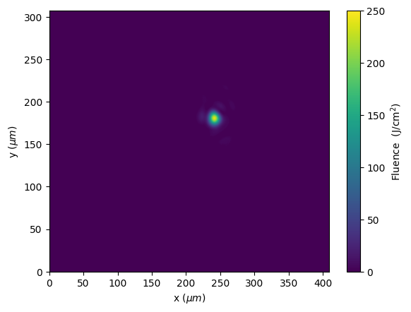
Plot the original transverse profile from the file. The laser occupies a small fraction of the image.
[8]:
fig, ax = plt.subplots()
cax = ax.imshow(
    intensity_data,
    aspect="auto",
    extent=np.array([lo[0], hi[0], lo[1], hi[1]]) * 1e6,
)
color_bar = fig.colorbar(cax)
color_bar.set_label(r"Fluence  (J/cm$^2$)")
ax.set_xlabel("x ($ \\mu m $)")
ax.set_ylabel("y ($ \\mu m $)")
plt.show()
Combine longitudinal and transverse profiles#
[9]:
laser_profile_raw = CombinedLongitudinalTransverseProfile(
    wavelength=longitudinal_profile.lambda0,
    pol=polarization,
    laser_energy=energy_J,
    long_profile=longitudinal_profile,
    trans_profile=transverse_profile,
)
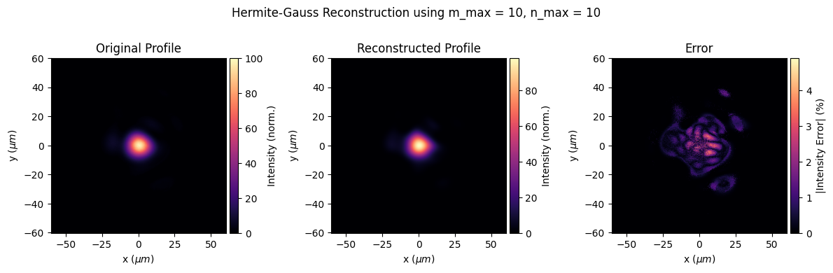
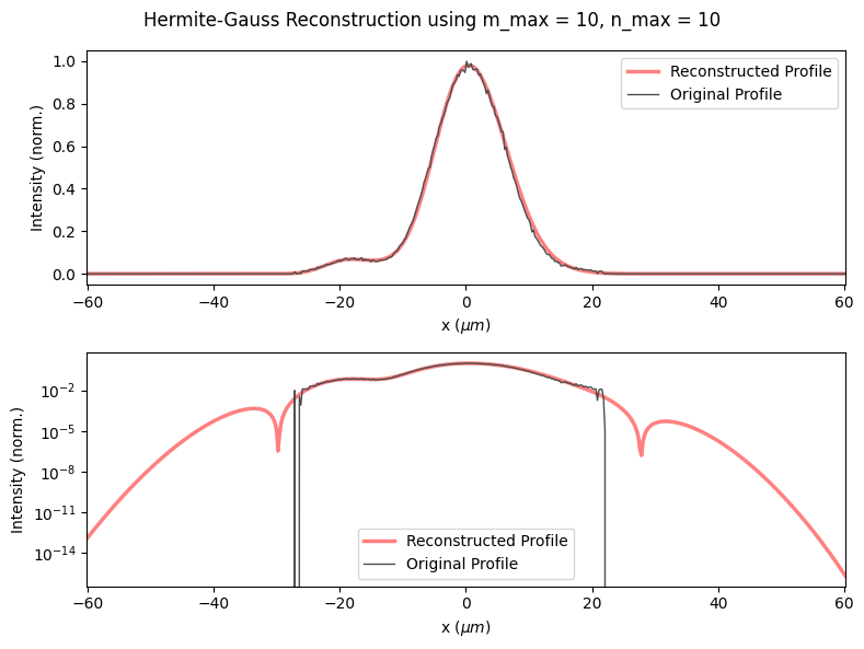
Clean/denoise the profile#
LASY functions can be used for denoising/cleaning. Here, the measured profile is decomposed into Hermite-Gauss modes. The cleaning is done by keeping only the first few modes. Take a look at the following example.
[10]:
# Maximum Hermite-Gauss mode index in x and y
m_max = 10
n_max = 10

# Calculate the decomposition and waist of the laser pulse
modeCoeffs, waistX, waistY = hermite_gauss_decomposition(
    transverse_profile,
    longitudinal_profile.lambda0,
    m_max=m_max,
    n_max=n_max,
    res=cal,
    lo=[-2e-4, -2e-4],
    hi=[2e-4, 2e-4],
)

# Create a num profile, summing over the first few modes
energy_frac = 0
for i, mode_key in enumerate(list(modeCoeffs)):
    tmp_transverse_profile = HermiteGaussianTransverseProfile(
        waistX, waistY, mode_key[0], mode_key[1], longitudinal_profile.lambda0
    )
    energy_frac += modeCoeffs[mode_key] ** 2  # Energy fraction of the mode
    if i == 0:  # First mode (0,0)
        laser_profile_cleaned = modeCoeffs[
            mode_key
        ] * CombinedLongitudinalTransverseProfile(
            longitudinal_profile.lambda0,
            polarization,
            longitudinal_profile,
            tmp_transverse_profile,
            laser_energy=energy_J,
        )
    else:  # All other modes
        laser_profile_cleaned += modeCoeffs[
            mode_key
        ] * CombinedLongitudinalTransverseProfile(
            longitudinal_profile.lambda0,
            polarization,
            longitudinal_profile,
            tmp_transverse_profile,
            laser_energy=energy_J,
        )

# Energy loss due to decomposition
energy_loss = 1 - energy_frac
print(f"Energy loss: {energy_loss * 100:.2f}%")
Estimated w0(x-axis) = 12.03 microns (1/e^2 width)
Estimated w0(y-axis) = 10.73 microns (1/e^2 width)
Energy loss: 1.73%
[11]:
# Plot the original and denoised profiles
# Create a grid for plotting
x = np.linspace(-5 * waistX, 5 * waistX, 500)
X, Y = np.meshgrid(x, x)

# Determine the figure parameters
fig, ax = plt.subplots(1, 3, figsize=(12, 4), tight_layout=True)
fig.suptitle(
    "Hermite-Gauss Reconstruction using m_max = %i, n_max = %i" % (m_max, n_max)
)
pltextent = np.array([np.min(x), np.max(x), np.min(x), np.max(x)]) * 1e6  # in microns
cbar_labels = ["Intensity (norm.)", "Intensity (norm.)", "|Intensity Error| (%)"]
title = ["Original Profile", "Reconstructed Profile", "Error"]
scale = ["linear", "log"]
lw = [1.0, 2.5]


# Original profile
prof1 = np.abs(laser_profile_raw.evaluate(X, Y, 0)) ** 2
maxInten = np.max(prof1)
prof1 /= maxInten

# Reconstructed profile
prof2 = np.abs(laser_profile_cleaned.evaluate(X, Y, 0)) ** 2
prof2 /= maxInten

# Normalized error
prof3 = (prof1 - prof2) / np.max(prof1)
prof = [prof1, prof2, prof3]

fig2, ax2 = plt.subplots(2, 1, figsize=(8, 6), tight_layout=True)
fig2.suptitle(
    "Hermite-Gauss Reconstruction using m_max = %i, n_max = %i" % (m_max, n_max)
)

for i in range(3):
    divider = make_axes_locatable(ax[i])
    ax_cb = divider.append_axes("right", size="5%", pad=0.05)
    pl = ax[i].imshow(100 * np.abs(prof[i]), cmap="magma", extent=pltextent)
    cbar = fig.colorbar(pl, cax=ax_cb)
    cbar.set_label(cbar_labels[i])
    ax[i].set_xlim(pltextent[0], pltextent[1])
    ax[i].set_ylim(pltextent[2], pltextent[3])
    ax[i].set_xlabel("x ($ \\mu m $)")
    ax[i].set_ylabel("y ($ \\mu m $)")
    ax[i].set_title(title[i])
    if i < 2:
        ax2[i].plot(
            x * 1e6,
            prof2[int(len(x) / 2), :],
            label=title[1],
            color=(1, 0.5, 0.5),
            lw=2.5,
        )
        ax2[i].plot(
            x * 1e6,
            prof1[int(len(x) / 2), :],
            label=title[0],
            color=(0.3, 0.3, 0.3),
            lw=1.0,
        )
        ax2[i].legend()
        ax2[1].set_yscale(scale[i])
        ax2[i].set_xlim(pltextent[0], pltextent[1])
        ax2[i].set_xlabel("x ($ \\mu m $)")
        ax2[i].set_ylabel("Intensity (norm.)")

plt.show()
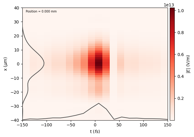
Create a laser#
Now the hard part is done! From the cleaned profile, we create a LASY Laser object (3D cartesian or cylindrical geometry) and write to a file compliant with the openPMD standard.
[12]:
# First, 3D geometry
dimensions = "xyt"  # Use 3D geometry
lo = (-40e-6, -20e-6, -150e-15)  # Lower bounds of the simulation box
hi = (40e-6, 20e-6, 150e-15)  # Upper bounds of the simulation box
num_points = (
    50,
    50,
    20,
)  # Number of points in each dimension. Use (300, 300, 200) for production.

# Constructing the object using 3D geometry might take a while to run depending on the hardware used.
laser_xyt = Laser(dimensions, lo, hi, num_points, laser_profile_cleaned)  # Laser
laser_xyt.normalize(energy_J * energy_frac)  # Normalize the laser energy
laser_xyt.show()

# Save the laser object to a file
laser_xyt.write_to_file("Laser_xyt_denoised", "h5", save_as_vector_potential=True)
[13]:
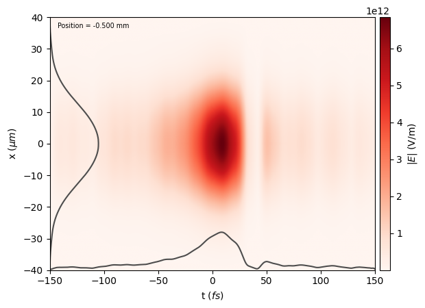
# Then, cylindrical geometry. Here, we also propagate the pulse backwards by 0.5 mm.
dimensions = "rt"  # Use cylindrical geometry
lo = (0, -150e-15)
hi = (40e-6, 150e-15)
num_points = (500, 400)

laser = Laser(dimensions, lo, hi, num_points, laser_profile_cleaned)
laser.normalize(energy_J * energy_frac)
laser.propagate(-0.5e-3)  # Propagate the laser pulse backwards
laser.show()

# Save the laser object to a file
laser.write_to_file("Laser_rt_propagated", "h5", save_as_vector_potential=True)
Available backends are: NP
NP is chosen